1 Overview
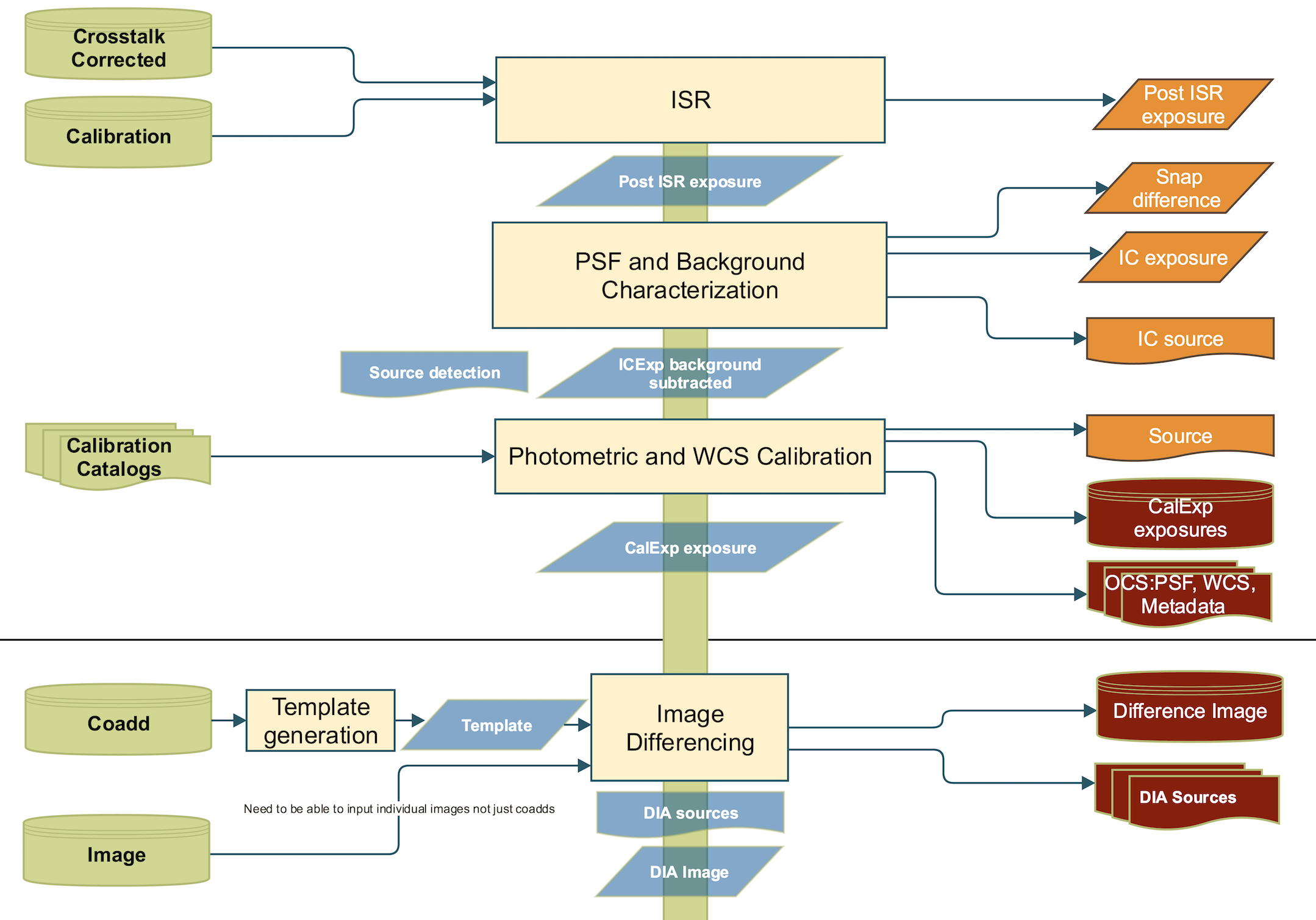
Ultimately, LSST Alert Production (AP) will need to perform all steps of the Level 1 pipeline automatically on each new raw image from the telescope. Details are in the LSST Data Management Science Pipelines Design (LDM-151, [swi17]) and the LSST Data Products Definition Document (DPDD, [jur16]). Briefly summarized below and in Figure 1, the first portion of these steps are:
- Instrument Signature Removal (ISR), which includes crosstalk and linearity corrections, bad pixel masking, bias subtraction, and flat field division,
- Point Source Function (PSF) and background characterization, which includes source detection and measurement,
- Photometric and World Coordinate System (WCS) calibration, and
- Image Differencing with an appropriate template (which may need constructing) to create Difference Image Analysis (DIA) source catalogs.

Figure 1 The first portion of the Nightly Processing Pipeline overview, from Figure 1 of LDM-151 [swi17]. This encompasses all of “Single Frame Processing” and part of “Alert Detection.”
A number of packages in the LSST Software Stack have been developed to perform portions of one or more of these four tasks, but they are not yet linked together in an automated way. This Prototype AP Pipeline is the first step toward the goal of an automatic Level 1 Pipeline that can process a set of raw images through each of these steps and verify that the output is what we expect.
2 Dataset
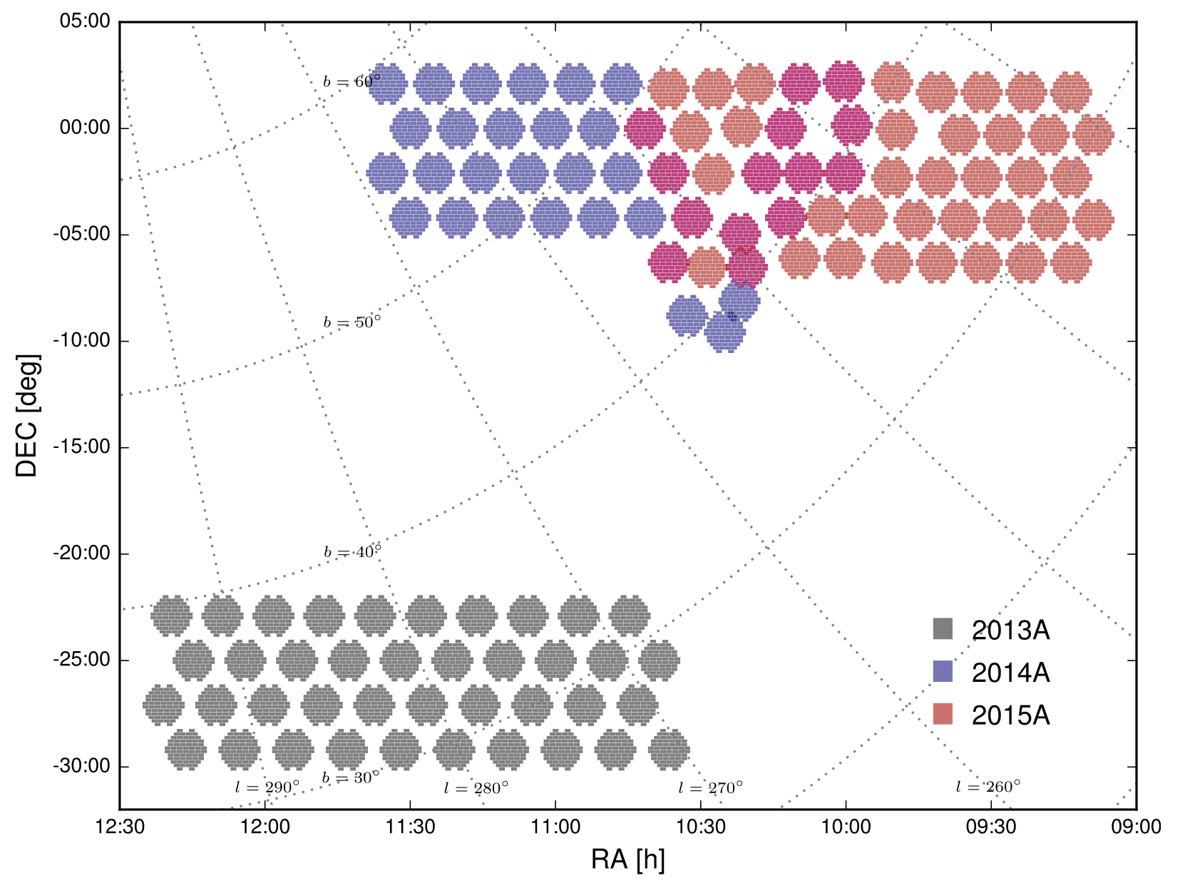
We use images from the High Cadence Transient Survey (HiTS, [for16]), a three-year survey from 2013–2015 which used the Dark Energy Camera (DECam) on the 4 m Blanco telescope at Cerro Tololo Interamerican Observatory (CTIO). The primary science goal of this survey is to detect and follow up optical transients that have characteristic timescales from hours to days, with a particular interest in catching early supernovae. The distribution of the HiTS survey fields in the sky is shown in Figure 2.

Figure 2 Spatial distribution of the fields observed in the 2013–2015 HiTS campaign (Figure 4 from [for16]). The fields selected for this dataset are three of the pink ones, which indicate they were visited in both 2014 and 2015.
We select HiTS fields Blind15A_38, Blind15A_39, and Blind15A_40, which
are repeat observations of the same region of sky as Blind14A_07, Blind14A_08, and Blind14A_10
fields, respectively. They are all centered near an RA of 10:15:00 hr and Declination of –04:00:00 deg.
Each field has 34–36 individual visits over about a month, and each DECam image consists of 62 CCDs.
Most of the visits are in the g-band, some are in the r-band, and a few are in z or i.
For the purposes of this prototype pipeline, we consider two g-band visits in Blind15A_38 only.
However, the rest of the visits in fields 15A_38–15A_40 have been ingested (see details in Method)
and are ready for the next steps of processing if desired.
3 Method
To begin, we obtained the dataset by downloading raw images and corresponding master calibration files
from the NOAO Science Archive. The HiTS survey data
may be selected by searching for PI Förster. Additionally, the latest set of DECam defects (bad
pixel masks) were obtained from the lsst-dev server at /datasets/decam/calib/bpmDes/2014-12-05/,
and a set of Pan-STARRS astrometric reference catalogs were obtained from
the lsst-dev server at /datasets/refcats/htm/htm_baseline.
Next, we ran four main processing steps with the LSST Stack on the data:
ingestImagesDecam.py, from theobs_decampackage but drawing heavily onpipe_tasks,ingestCalibs.py, from thepipe_taskspackage,processCcd.py, from thepipe_taskspackage, andimageDifference.py, also from thepipe_taskspackage.
To streamline this process, we wrote a python script called decam_process.py to handle each step.
It is available on GitHub.
While it was only used on the Dataset described above, it can
in principle be applied to any set of raw DECam images using the LSST Stack, as shown below.
3.1 Tutorial
The prerequisites for running the Prototype Pipeline on a dataset of images (*.fits or *.fits.fz) are:
- The LSST Stack with the standard modules (
setup lsst_apps), as well asobs_decam(setup obs_decam) - A directory containing some raw DECam images, available from the NOAO Science Archive
- A directory containing DECam MasterCal biases and flats corresponding to the raw images, also available from the the NOAO Science Archive
- A directory containing DECam defect images, one for each CCD, available on the
lsst-devserver at/datasets/decam/calib/bpmDes/2014-12-05/ - A set of astrometric reference catalogs (example below)
- A personal working copy of the decam_process script
To begin, edit the values near the top of the decam_process script to reflect your desired directory names
for where processed images will live, as well as to specify the visits and CCDs you wish to process. The default presets are
repo = 'ingested_15A38/'  # used by ingest, ingestCalibs, processCcd
calibrepo = 'calibingested_15A38/'  # used by ingestCalibs, processCcd
processedrepo = 'processed_15A38/'  # used by processCcd, diffIm
diffimrepo = 'diffim_15A38_g/'  # used by diffIm
visits = [410927, 411033]  # used by processCcd, diffIm
# NOTE: visits assumes the first element is template and the rest are science
ccdnum = '1..62'  # used by processCcd, diffIm
# NOTE: the default '1..62' value includes all of the DECam CCDs
In general, repo refers to where ingested images will live, calibrepo
refers to where ingested calibration products (flats and biases) will live, processedrepo refers to where “calexp”
images will live (i.e., those that have been processed with processCcd including steps 1 through 3 in Overview),
and diffimrepo refers to where difference images and DIA Sources (catalogs) will ultimately live.
These should each be different directories, and it’s recommended to have them all reside in the same top-level directory.
Visit numbers can be found in image headers or retrieved from the registry database created in repo during image ingestion
(visit numbers are not used during ingestion, so you may set them after this step). The first visit you specify
in the list will be used as the template.
Finally, copy or link the Pan-STARRS astrometric reference catalog into the directory you’ve chosen for
repo and call it ref_cats. If you are working on the lsst-dev server, you can link the Gaia,
Pan-STARRS, and SDSS catalogs by
mkdir repo ln -s /datasets/refcats/htm/htm_baseline repo/ref_cats
Note that the repo directory is called ingested_15A38 in the default values given above.
If you wish to use an astrometric reference catalog other than Pan-STARRS, you must update the code in the doProcessCcd
function of decam_process.py accordingly. It is not necessary to explicitly mkdir the other repositories.
If you really don’t want to deal with astrometric reference catalogs, you can skip the astrometry and
photometric calibration steps by editing the contents of args in the doProcessCcd function of decam_process.py.
In this situation, you would set both calibrate.doAstrometry=False and calibrate.doPhotoCal=False.
Be aware that the difference imaging will not work well in this case, however, because the visits
will not be precisely lined up to the same WCS.
Once you are ready, run the following:
- Ingest the raw images
python decam_process.py ingest -f path/to/rawimages
- Ingest the calibration products (biases, flats, and defects)
python decam_process.py ingestCalibs -f path/to/biasesandflats -d path/to/defects
3. Run processCcd to detect PSF sources, characterize the background, and perform photometric and astrometric calibrations.
The end result of this step is calibrated exposures (“calexp” images). If you turned off photometric and astrometric calibrations
as described above, this step will still produce calexps, they will just not be precisely aligned from one visit to the next.
python decam_process.py processCcd
- Finally, do difference imaging using the first visit as the template
python decam_process.py diffIm
4 Results
The final difference images and DIA Source catalogs for the test dataset are available
on the lsst-dev server at /project/mrawls/prototype_ap/diffim_15A38_g/deepDiff/v411033/.
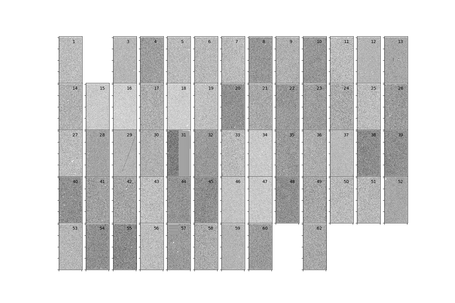
A small thumbnail preview of the difference images is shown in Figure 3.
Future work will extend this to more visits, perhaps using the 2014 visits as templates and the 2015 visits as science. This Prototype Pipeline will be used as a core component of the AP Minimum Viable System with a goal of verifying the different components of LSST image processing as we incrementally build toward a fully functional AP system.

Figure 3 Difference images for HiTS field Blind15A_38 with visit 410927 as the template
image and visit 411033 as the science image. CCDs 2 and 61 are nonoperational, and
a portion of CCD 31 is also not working. The other CCDs all perform as expected.
| [for16] | (1, 2) Förster et al. 2016, ApJ, 832, 155. The High Cadence Transient Survey (HITS). I. Survey Design and Supernova Shock Breakout Constraints. |
| [jur16] | Jurić et al. 2016, LSST Document LSE-163. Large Synoptic Survey Telescope Data Products Definition Document. |
| [swi17] | (1, 2) Swinbank et al. 2017, LSST Document LDM-151. Large Synoptic Survey Telescope Data Management Science Pipelines Design. |